Адрес первоисточника:
http://www.acadjournal.com/2002/v8/part1/p1/index.html
DISCRETE FAST WAVELET TRANSFORM ALGORITHM
AND ITS APPLICATION TO PREDICTION PROBLEM
Zaharov V.V., Fausto Casco S.
Universidad Autonoma Metropolitana - Iztapalapa,
Av. Michoacan y Purisima, Colonia Vicentina, C.P.09340,
México D.F., MEXICO,
Tel. (5255)58044637, vick@xanum.uam.mx
Abstract: Method of nonstationary stochastic process prediction using discrete wavelet transform is presented. As it is shown, the application of Discrete Wavelet Transform in maximum entropy prediction method allows decrease the square average prediction error in comparison with conventional methods that use algorithm of Discrete Fourier Transform approximately 3-4 times for presented test sequence. Its advantage was obtained due to information about process structure in the varied bands of frequency that received from coefficients of Discrete Wavelet Transform.
Keywords: discrete wavelet transform, in maximum entropy prediction method, multiresolution analysis.
INTRODUCTION
Within recent years, increasingly Discrete Wavelet Transform (DWT) have been used in many real applications because it allows to present nonstationary process more adequately. The Fourier transform (FT) had wide application as a tool for data processing in many applications for many years. The bases of complex exponents used in Discrete Fourier Transform (DFT) is optimal as to the many criteria in case of stationary process since whereat the coefficients of decomposition are uncorrelated. In case of nonstationary process they lose localization in time domain. The analysis of such signals is possible with the DFT using sliding window through the data [8]. The disadvantage of such approach is the high computational complexity of the decomposition algorithm.
In DWT instead of harmonic orthogonal functions are used the systems of functions generated by shifts and the compression of some generating functions with compact support in frequency and time domains. That allows divide process on “small details” in frequency domain and in the same time to localize them in time domain. This "compact support" allows the wavelet transform (WT) to translate a time-domain function into a representation that is not only localized in frequency (like the FT) but in time as well.
Fundamentally,
wavelets are a new type of function, which provide an excellent orthonormal
basis for functions of one or more variables. They provide a localized basis,
and can represent square-integrable functions, but also constant and, more
generally, polynomial functions in a locally finite manner. In 1988 Daubechies'
fundamental paper on wavelets appeared [6]. In this paper was fined for the
first time a parameterised family of orthonormal systems of functions in ![]() with certain important complementary properties:
with certain important complementary properties:
1. Each system is generated from
a scaling function and a wavelet function by rescaling and translations, e.g., ![]() ,
,
![]() and the wavelet system
and the wavelet system ![]() is
an orthonormal basis for
is
an orthonormal basis for ![]() .
.
2. Each element in a given system has compact support in time and frequency domain. The supports of the basis functions becomes very small for large scaling index j.
3. There are fast algorithms for computing the coefficients of wavelet transform
4. The classical discrete Fourier and cosine transforms appear as a special case of the general discrete wavelet transform (DWT).
The aim of the proposed work is applying DWT to the prediction of nonstationary stochastic process of the various nature and comparative analysis of obtained prediction with traditional methods like the maximum entropy method [7,8] in which is used the spectral Fourier coefficients. In traditional methods was obtained the Fourier coefficients with data sliding window and without data sliding window.
I. SCALING AND WAVELETS FUNCTIONS
The main problem
of the wavelets analysis is creating of basis functions for wavelets systems
[1,2,9]. The synthesis of bases function is founded on the theory of
multiresolution analysis (MA) [10,11]. The sequence of closed subspaces ![]() of
of ![]() , is defined as a multiresolution
analysis of
, is defined as a multiresolution
analysis of ![]() if are
satisfied the following properties:
if are
satisfied the following properties:
1. ![]()
2. ![]() ,
,
3. ![]() ,
,
4. If ![]()
5.Such function ![]() (scaling
function) with a non-vanishing integral exists, that the collection of
his shifts
(scaling
function) with a non-vanishing integral exists, that the collection of
his shifts ![]() is a
orthonormal basis of
is a
orthonormal basis of ![]() .
.
Since ![]() a sequence hk exists such that the scaling function satisfies
the condition
a sequence hk exists such that the scaling function satisfies
the condition
![]() (1)
(1)
The equation (1) is refinement equation (or two scale difference equation).
The Fourier transform of the scaling function is
![]()
where ![]() is a 2p -periodic function.
is a 2p -periodic function.
By integrating both sides of
eq.(1), and dividing by the non-vanishing integral of j , we see that ![]() ,
and as a consequence
,
and as a consequence ![]() .
.
The scaling function meets the
normalization condition ![]() and
for its collection
and
for its collection ![]() [2].
[2].
The collection of functions
![]() (2)
(2)
is the orthonormal basis of the
space![]() .
.
In many applications, we never
need the scaling function itself. Instead we may often work directly with the hk.
An orthogonal scaling function is a function j such that the set ![]()
![]() is an orthonormal basis and
satisfies by the next property
is an orthonormal basis and
satisfies by the next property
![]() (3)
(3)
With such j , the collection of
functions ![]() is an
orthonormal basis of
is an
orthonormal basis of ![]() and
the collection of functions
and
the collection of functions ![]() is an orthonormal basis of
is an orthonormal basis of ![]() .
.
Using the Poisson summation formula [10], in the frequency domain we have
![]()
We consider the
subspace ![]() as complementary
space of
as complementary
space of ![]() in
in ![]() ,
,
![]() . If the set
. If the set ![]() consists on functions which spectrums are concentrated in interval
consists on functions which spectrums are concentrated in interval ![]() ,
then
,
then ![]() consists on the
function with spectrum in interval
consists on the
function with spectrum in interval ![]() and
and
![]() , symbol Å is direct
sum sign. In other words, each element of
, symbol Å is direct
sum sign. In other words, each element of ![]() can be written as the sum
can be written as the sum ![]() .
The space
.
The space ![]() contains the
detail information needed to go from an approximation at resolution j to
an approximation at resolution j+1. Consequently,
contains the
detail information needed to go from an approximation at resolution j to
an approximation at resolution j+1. Consequently, ![]() .
.
A function ![]() is a wavelet if the collection of his shifts
is a wavelet if the collection of his shifts ![]() is a orthonormal basis of
is a orthonormal basis of ![]() and
the collection of functions
and
the collection of functions
![]() (4)
(4)
is orthonormal basis of ![]() .
.
Each element in a given system
has compact support in time and frequency. Since the wavelet ![]() a sequence gk exists such that
a sequence gk exists such that
![]() , (5)
, (5)
where ![]() and
and ![]() , ¾ is the sign
of conjugation.
, ¾ is the sign
of conjugation.
The Fourier transform of the wavelet is given by
![]() ,
,
where ![]() is a 2p -periodic function and
is a 2p -periodic function and ![]() .
.
An orthogonal wavelet is a
function y such that the collection of functions ![]()
![]() is an orthonormal basis of
is an orthonormal basis of ![]() .
In this case
.
In this case
![]() .
(6)
.
(6)
In the frequency domain eq. (6)
is ![]() .
.
The collection of functions ![]() is an orthonormal basis of
is an orthonormal basis of ![]() .
Since the spaces
.
Since the spaces ![]() are
mutually orthogonal, the collection of functions
are
mutually orthogonal, the collection of functions ![]() is an orthonormal basis of L2(R).
is an orthonormal basis of L2(R).
Than, a sufficient condition for
a multiresolution analysis to be orthogonal is ![]()
![]() .
(7)
.
(7)
The same in the frequency domain
![]() , (8)
, (8)
2. FAST WAVELET TRANSFORM
The decomposition of any given
function in space![]() can be presented as
can be presented as
![]() (9)
(9)
where  .
.
Taking into account that ![]() and
applying of eq.(9) we write
and
applying of eq.(9) we write
![]() (10)
(10)
Lemma:
![]() can be presented as
can be presented as ![]() ;
;
![]() can be presented as
can be presented as ![]()
Demonstration:
Similarly for ![]() .
.
Multiplicating (10) at ![]() and
applying eq.(3) , (7) and lemma we get
and
applying eq.(3) , (7) and lemma we get
![]() ½ ´
½ ´
![]()

Multiplicating (10) at ![]() and applying eq.(6)we get
and applying eq.(6)we get

In general case ![]() and we have equation
and we have equation
![]() (11)
(11)
From eq.(11) the coefficients ![]() and
and ![]() can be define as
can be define as
![]() ;
; ![]() j=-1,-2,…,-m
j=-1,-2,…,-m
Replacing ![]() y
y ![]() we get
we get
![]() ;
; ![]() j=-1,-2,…,-m (12)
j=-1,-2,…,-m (12)
The eq. (12) is
direct discrete fast wavelet transform that consists from 2 convolutions, and ![]() is initial coordinates of any function in the space
is initial coordinates of any function in the space![]() ,
where
,
where ![]()
Applying the similar manner by
multiplying (11) at ![]() we
have
we
have
![]()
Therefore we have inverse fast wavelet transform
![]() (13)
(13)
One of the powers of wavelet technology is the ability to choose the defining coefficients for a given wavelet system to be best adapted to the given problem. Daubechies developed in her original paper [6] specific families of wavelet systems which had maximal vanishing moments of the function and which were very good for representing polynomial behavior.
3. PYRAMIDAL STRUCTURE OF THE WAVELET TRANSFORM
As follows from (12) and (13) the forward and inverse wavelet transform can be implemented using a set of upsamplers, downsamplers and recursive two-channel filter banks, that named also pyramidal algorithm because has pyramidal structure. At [1,5] has shown that the tree or pyramid algorithm can be applied to the wavelet transform by using the wavelet coefficients for calculate the filter coefficients of the QMF (Quadrature Mirror Filter) filter pairs. From relation (8) follows that for the filter coefficients have the following properties in frequency domain
![]() ;
;
![]() ;
;
![]() ;
;
![]()
The same wavelet
coefficients are used in both the low-pass (LP) and high-pass (HP) (actually,
band-pass) filters. The low-pass filter coefficients ![]() are associated with the scaling function. The output of each low-pass filter is
are associated with the scaling function. The output of each low-pass filter is ![]() ,
or approximation components, of the original signal for that level of the tree.
The high-pass filter coefficients
,
or approximation components, of the original signal for that level of the tree.
The high-pass filter coefficients ![]() is associated with the wavelet function (note the alternating sign change)
is associated with the wavelet function (note the alternating sign change) ![]() .
.
The output of
each high-pass filter is the ![]() ,
,![]() or detail components, of the original signal. The
or detail components, of the original signal. The ![]() of the previous level are used to generate the new
of the previous level are used to generate the new ![]() and
and ![]() for the next level of
the tree. Decimation by two corresponds to the multiresolution nature (the j
parameter) of the scaling and wavelet functions (see Figure 1).
for the next level of
the tree. Decimation by two corresponds to the multiresolution nature (the j
parameter) of the scaling and wavelet functions (see Figure 1).
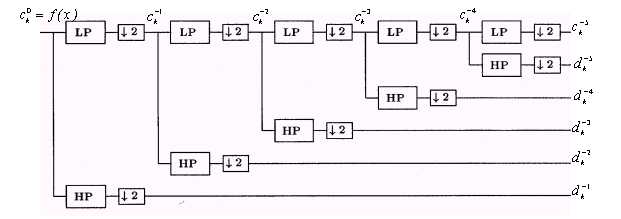
Figure 1. Direct pyramidal structure
The reverse fast
wavelet transform essentially performs the operations associated with the
forward fast wavelet transform in the opposite direction (Figure 2). The
expansion coefficients are combined to reconstruct the original signal. The
same ![]() ,
,![]() coefficients are used as in the forward transform, but in reversed order. The
process works down the branches of the tree combining the approximation and
detail signals into approximation signals with higher levels of detail.
coefficients are used as in the forward transform, but in reversed order. The
process works down the branches of the tree combining the approximation and
detail signals into approximation signals with higher levels of detail.
Instead of decimation, the signals are interpolated: zero’s are placed between each approximation and detail sample, and the signals are then passed through the low-pass and high-pass filters. The intermediate 0 values are replaced by "estimates" derived from the convolutions. The filters' outputs are then summed to form the approximation coefficients for the next higher level of resolution. The final set of approximation coefficients at the tree's top level in the reverse transform is a reconstruction of the original signal data points.
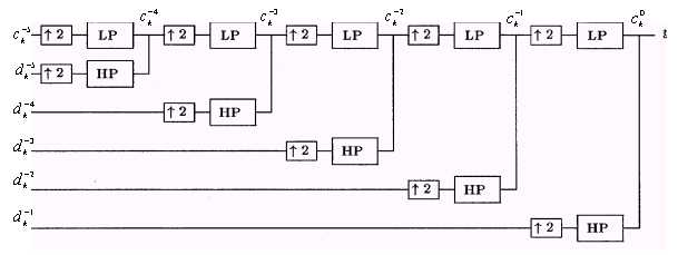
Figure 2. Inverse pyramidal structure
As follows from
eq.(12) and (13) the signal decomposition depends on the impulse responses of
the low and high pass filters, that in turn depends on the choosing of scaling
and wavelets function. The function ![]() and
and ![]() can be interpreted as
coefficients of the series for the functions
can be interpreted as
coefficients of the series for the functions ![]() and
and ![]() and have the forms
and have the forms
![]() (14)
(14)
![]() (15)
(15)
In signal processing terminology, the various bases of the DWT can be used by choosing the corresponding coefficients of filter banks.
4. DWT APPLICATION FOR PREDICTION PROBLEM
We consider applying DWT for prediction problem. As the basic method will be used the maximum entropy method [7,8] in which instead of spectral Fourier coefficients have been used the coefficients of DWT calculated according to eq.(12).
The first application of DWT for linear prediction system was proposed in [4]. The concept behind this system is to use the DWT to decompose the data into "subspaces" that are easier to model with multiple linear predictors. The paper [12] considers the DWT application for market stock rate analysis some of the nonstationary data.
We will use the classical method of prediction using AR- model for an estimation of a forward linear prediction of element xn, n =1,2...,N and xn = 0 at n < 1, n > N
![]() ,
(16)
,
(16)
where ![]() is estimation of element of xn , ak is a
coefficients of prediction filter, N is number of elements of a time
series, p is order of AR - model.
is estimation of element of xn , ak is a
coefficients of prediction filter, N is number of elements of a time
series, p is order of AR - model.
If minimize an
error of a linear prediction ![]() ,
then a vector of a linear prediction parameters ak which
minimizes the average square of an error
,
then a vector of a linear prediction parameters ak which
minimizes the average square of an error ![]() is the solution of the normal equations
is the solution of the normal equations
![]() ,
(17)
,
(17)
where ![]() is (p + 1) vector,
is (p + 1) vector, ![]() ,
,![]() ,
,
![]() , ~ is symbol of transpose
and conjugate, T is transpose symbol,
, ~ is symbol of transpose
and conjugate, T is transpose symbol, ![]() is Toeplitz (p+1)´ (p+1) correlation matrix of input
data, X is (N+p)´ (p+1) matrix of input data with
structure as shown below
is Toeplitz (p+1)´ (p+1) correlation matrix of input
data, X is (N+p)´ (p+1) matrix of input data with
structure as shown below
 (18)
(18)
The eq.(17) is the Yule- Walker equation for autoregressive process and can be solved concerning to parameters ai, i=1,2..., p by various known algorithms, for example by Levinson algorithm [1]. In particularly if the inverse matrix has a form
 (19)
(19)
then the solution of eq.(17) is
 (20)
(20)
The solution (17) allows obtaining the spectral density of input data for the received parameters with maximum entropy [1]
 (21)
(21)
were ![]() is estimation of parameter an, , D
t is a sampling interval.
is estimation of parameter an, , D
t is a sampling interval.
For prediction of nonstationary sequences more referable introduce the exponential window that is gone along the input data, creating the least change of the current errors and very strongly reducing of older ones. Thus the equation for r we put as
![]() ,
(22)
,
(22)
were w is positive real scalar satisfying to a condition 0 < w £ 1. Then expression for a matrix R we can write
![]() ,
(23)
,
(23)
where ![]() is
n-th row of matrix X , n = 1,2..., N+p.
is
n-th row of matrix X , n = 1,2..., N+p.
We will consider and then compare for criteria of minimum prediction errors 3 basic algorithm of prognostications
Algorithm1. Classical method of prediction without sliding window, that consists from the following steps:
Step 1. Obtaining of current input data element xn, n=1,2,…,N
Step 2. Forming matrix of input data X according of eq.(18)
Step 3.
Calculation of a matrix ![]() and
vector A using eq.(19) and (20).
and
vector A using eq.(19) and (20).
Step 4. Estimation of a forward linear prediction of elements xn with eq. (16)
Algorithm2. Classical method of prediction with sliding window, that consists from the following steps:
Step 1. Obtaining of current input data element xn, n=1,2,…,N
Step 2. Forming and waiting of (N+p)´ (p + 1) input data matrix X
![]() (24)
(24)
where ![]() ,
n = 1,2, …, N +p is number of the current element.
,
n = 1,2, …, N +p is number of the current element.
 (25)
(25)
Step 3.
Calculation of a matrix ![]() and
vector A using eq.(19) and (20).
and
vector A using eq.(19) and (20).
Step 4. Estimation of a forward linear prediction of elements xn with eq.(16).
Algorithm 3. Prediction algorithm that uses DWT.
Step 1. Obtaining of current input data element xn, n=1,2,…,N+p
Step 2. Calculating the DWT of the input data in the finite interval and defining the DWT coefficients.
![]() ;
; ![]() j=-1,-2,…,-m
(26)
j=-1,-2,…,-m
(26)
Step 3. Carrying out of forward linear prediction of wavelets coefficients for each level of scale.
![]() ,
(27)
,
(27)
![]() , (28)
, (28)
where the
coefficients ![]() of the
prediction filter determined similar as in eq.(20).
of the
prediction filter determined similar as in eq.(20).
Step 4. Obtaining the predicted data using inverse DWT with prediction coefficients.
![]() ,
(29)
,
(29)
where ![]() is
the initial prediction function.
is
the initial prediction function.
The variety of orthonormal bases which can be formed by the Discrete Wavelet Transform algorithm, coupled with the infinite number of wavelet and scaling functions which can be created, yields a very flexible analysis tool. Not only can the best wavelet be chosen to analyse a particular signal but the best orthonormal basis as well. But in many applications as shows the practice the Daubechies wavelets are optimum at concentrating the signal power into the lower-scale transform coefficients. As a result, there is less "risk" in the prediction.
To compare the presented algorithm on prediction problem the simulation in PC was carry out. For the evolution of prediction mean least square error e2(n) are used the sequence with 10 single tone components with frequencies since 1 Hz to 25 Hz with interval 2-7Hz with random initial phases on interval 0-2p and white noise with power 3 time less then complete power of tone components. To this process was added the trend component than simulated as a lineal polynomial function.
The prediction was made in 20 forward samples with using 3 algorithm of spectral coefficients obtaining: DWT (1), DFT with windowing (2) and DFT without windowing (3). In the experiment was evaluated relation e2(n)/ x2(n) for each of 20 forward samples. The result was averaged for 200 statistics and is shown in Figure 3.
Figure3. Depending of prediction error from the number of forward samples
As follows from figure3, applying DWT for prediction reduce the e2(n)/ x2(n) relation approximately three times in comparison with DFT with sliding window and four times without sliding window when the number of prediction samples equal 20.
5. CONCLUSION
In this paper the fast discrete wavelet transform and its application to prediction of nonstationary stochastic process was presented. As it is shown, the application of DWT in maximum entropy prediction method is allows decrease the square average prediction error in comparison with methods that using DFT with sliding window and DFT without sliding window. In particularly, for the presented test sequence for the number of prediction samples equal 20 the gain is 3-4 times in comparison with DFT prediction methods. Its advantage was obtained due to information about process structure in the varied bands of frequency that received from coefficients of DWT.
6. REFERENCES